Internalizing RoPE embeddings. If, like me, you slept under the rock since the introduction of RoPE in 2021 this document provides the most-brief late 2025 update on the latest practical tech. Jump start your paper reading here!

Minimal background and notations

Self-attention sublayer of the transformer block derives Query Key Value from each token in the sequence. Query of the target token would be compared to Key of preceding words to determine in which proportion Values of the previous tokens to be blended together using softmax function:

\[\text{softmax}_{n}\left(\frac{q^T_i k_n}{\sqrt{|D|}}\right), \text{where }i\in[0, n]\]

Positional embedding is the main way to help network distinguish between words at different positions. Softmax by itself does not distinguish tokens that close from those that are far. We used to provide position as an integer (lacking suitable representation in NN) or convert position index to a one-hot embedding, which wasted computational resources and was non-compositional.

RoPE: formula, transformation, computational advantage.

RoPE takes a 8192-dimensional embedding, partitions it into 4095 2D subspaces (2D pairs). Each subspace is assigned a rotation speed according to an exponential formula. When attention is calculated embedding of the Key is rotated by the rotation speed multiplied by the distance from the Query token.

Formula for rotation momentum depending on the subspace index $i\in[0, D/2]$:

\[\theta_i(p) = p \cdot Q^{- \frac{2i}{d}}\]

Let’s unpack it. If we start from embedding size $d=8192$ embedding subspace $i \in [{0, \dots, \tfrac{d}{2}-1}]$ (so, $[0, 4095]$). Token positions $p$ for a 6-token sequence when calculating attention for the 5th token would be $[3, 2, 1, 0, -, -]$. Base $Q$ is an arbitrary number and the original authors set it to $10000$.

Example: elements $[8,9]$ (out of 8192, subspace $i=4$) for token at position 15 would be rotated by $15 \cdot 10000^{-\frac{8}{8192}} = 15 \cdot 1.009 = 15.135$ radians. Which is about $867^{\circ}$ ($57.3^{\circ}$ per radian) and since we can ignore full rotation it is equivalent to $867\mod 360 = 147^{\circ}$.

The rotary embedding applied to the corresponding 2D subspace is:

\[\mathrm{RoPE}_i(p) = \begin{pmatrix} \cos \theta_i(p) & -\sin \theta_i(p) \\ \sin \theta_i(p) & \cos \theta_i(p) \end{pmatrix}\]

And the complete transformation matrix looks like this:

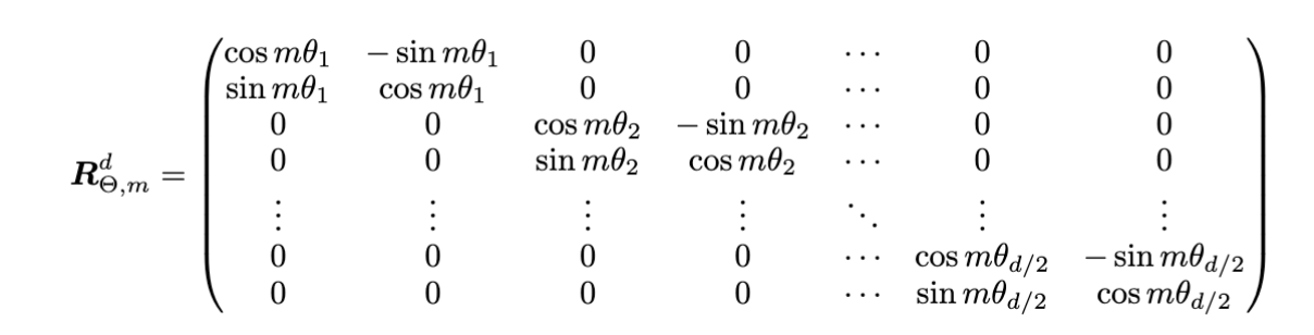
Su, Jianlin; Lu, Yu; Pan, Shengfeng; Wen, Bo; Liu, Yunfeng (2021) “RoFormer: Enhanced Transformer with Rotary Position Embedding” arXiv:2104.09864

RoPE authors make the following arbitrary choices setting up RoPE embedding:

• maximum rotation angle of 1 rad
• minimum rotation angle of $1/10000*rad$
• linearly exponential transition between minimum and maximum angle
• distance between tokens $(t_i,t_j)$ is measured as difference between indexes $i \text{ and } j$ $int(i-j)$

Recap:

• RoPE transforms embeddings without adding new dimensions or trainable parameters
• Rope partitions embedding space into 2D subspaces. In each subspace it rotates vectors by a unique angle. Angle is multiplied by integer distance.
• RoPE preserves embedding norm (true for every subspace)
• Original formulation allows for an efficient implementation where Q for each token is projected exactly once.

RoPE has one major limitation: performance of the model drops significantly if during inference distances $p$ exceed those seen in training.

Notation

• $D$ — size of the embedding space
• $i$ — rotary dimension index (each $i$ corresponds to one 2D plane)
• $p$ — token position index (0-based or 1-based; consistent choice assumed)
• $L_{\mathrm{train}}$ — maximum context length seen during training
• $L_{\mathrm{target}}$ — desired inference-time context length
• $Q$ — RoPE base (commonly $10{,}000$)
• $\alpha$ — NTK scaling factor
  (often $\alpha = \tfrac{L_{\mathrm{target}}}{L_{\mathrm{train}}}$)
• $\theta_i(p)$ — rotation angle for dimension $i$ at position $p$
• $\mathrm{RoPE}_i(p)$ — $2 \times 2$ rotation matrix applied to query/key components

RoPE visualization

Let’s dwell a little on this transformation.

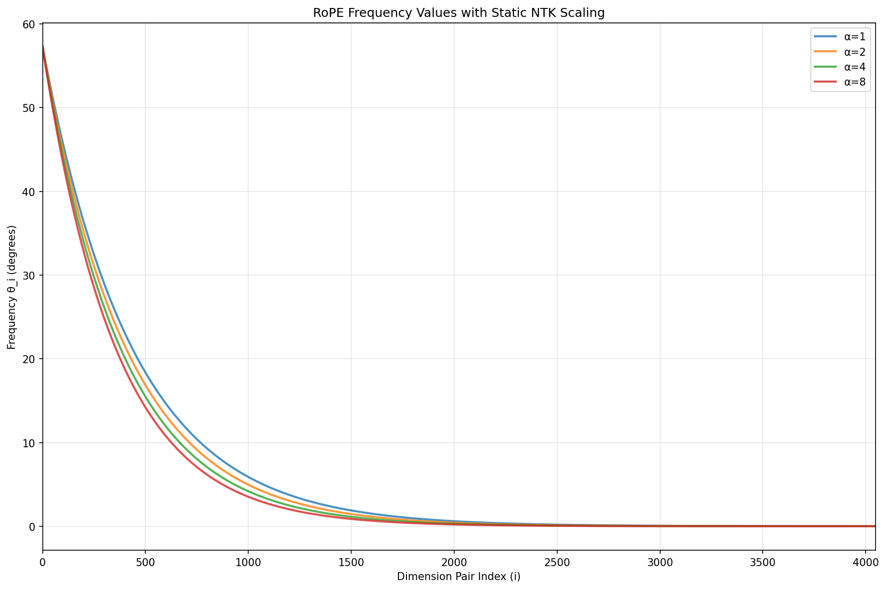
In practice here is how angle would change depending on the embedding component position $i$. I find degrees to be more intuitive than radians. I print values of $\theta$ as a bar chart and sort them by index $i$ since so far $i$ is in fact discrete.

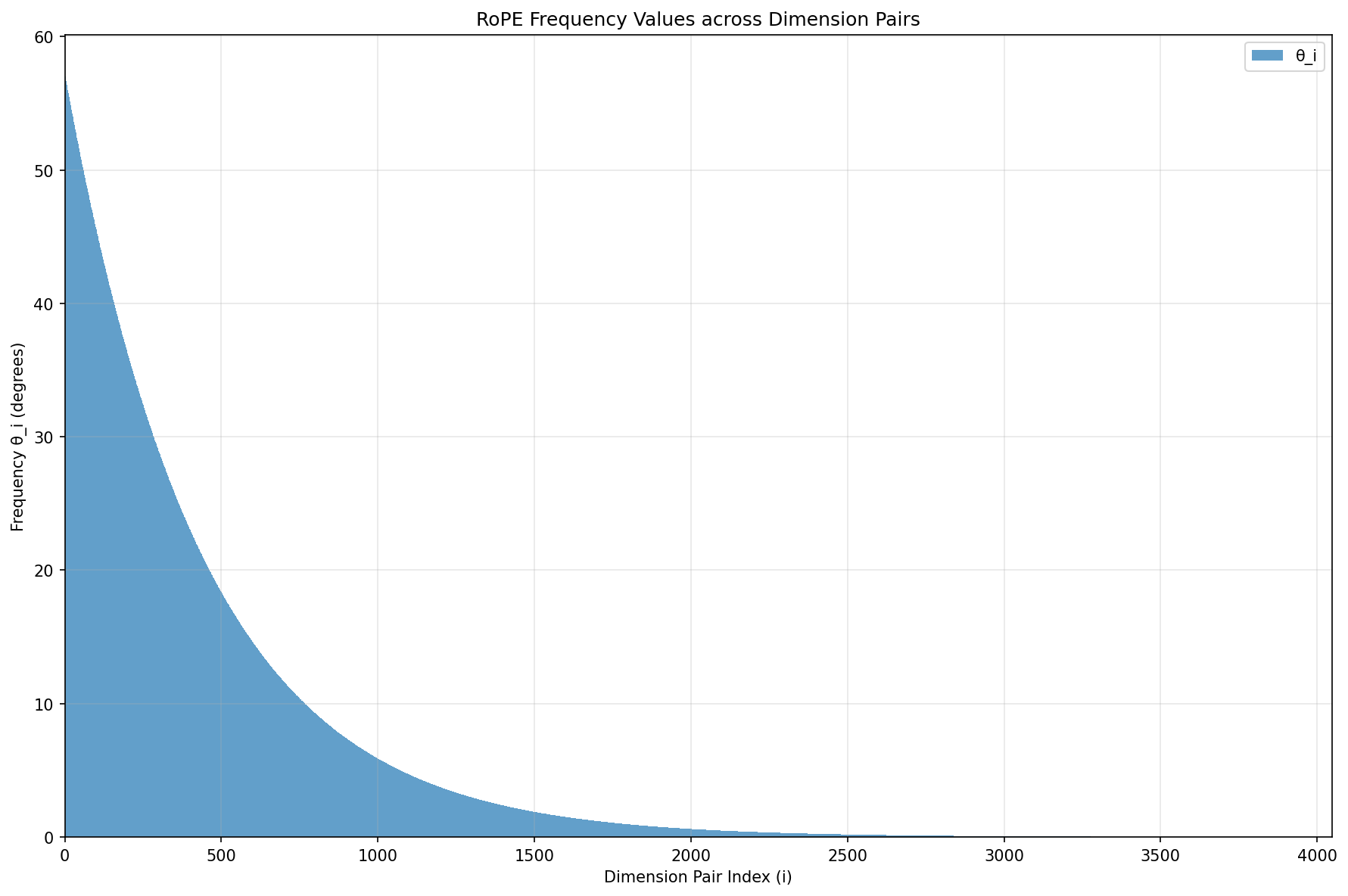
Observation: we rotate lower 100s of dims by 50-60 degrees while higher (>2000) dimensions rotations is hardly noticeable at low distances. Changing embedding size 2048 to 16386 the shape of the curve would remain the same, it would simply stretch over more indexes i.

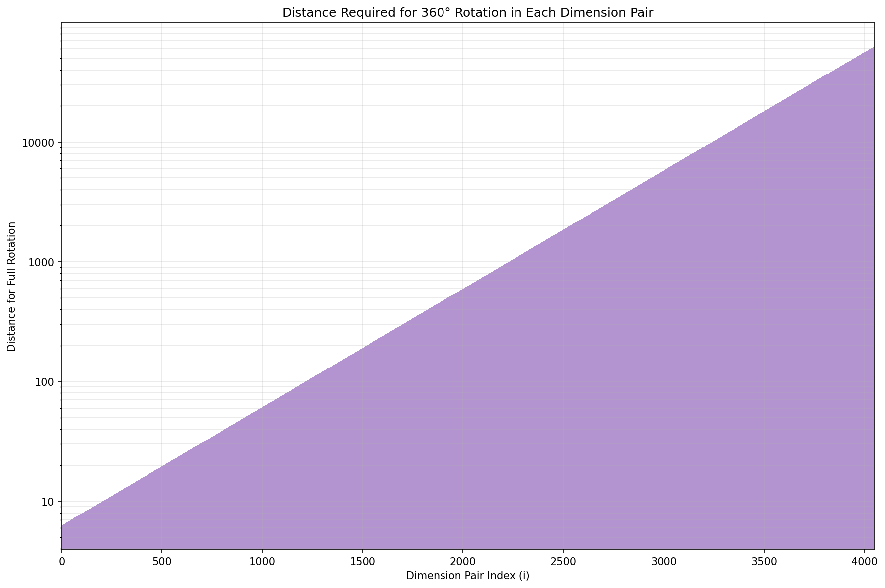
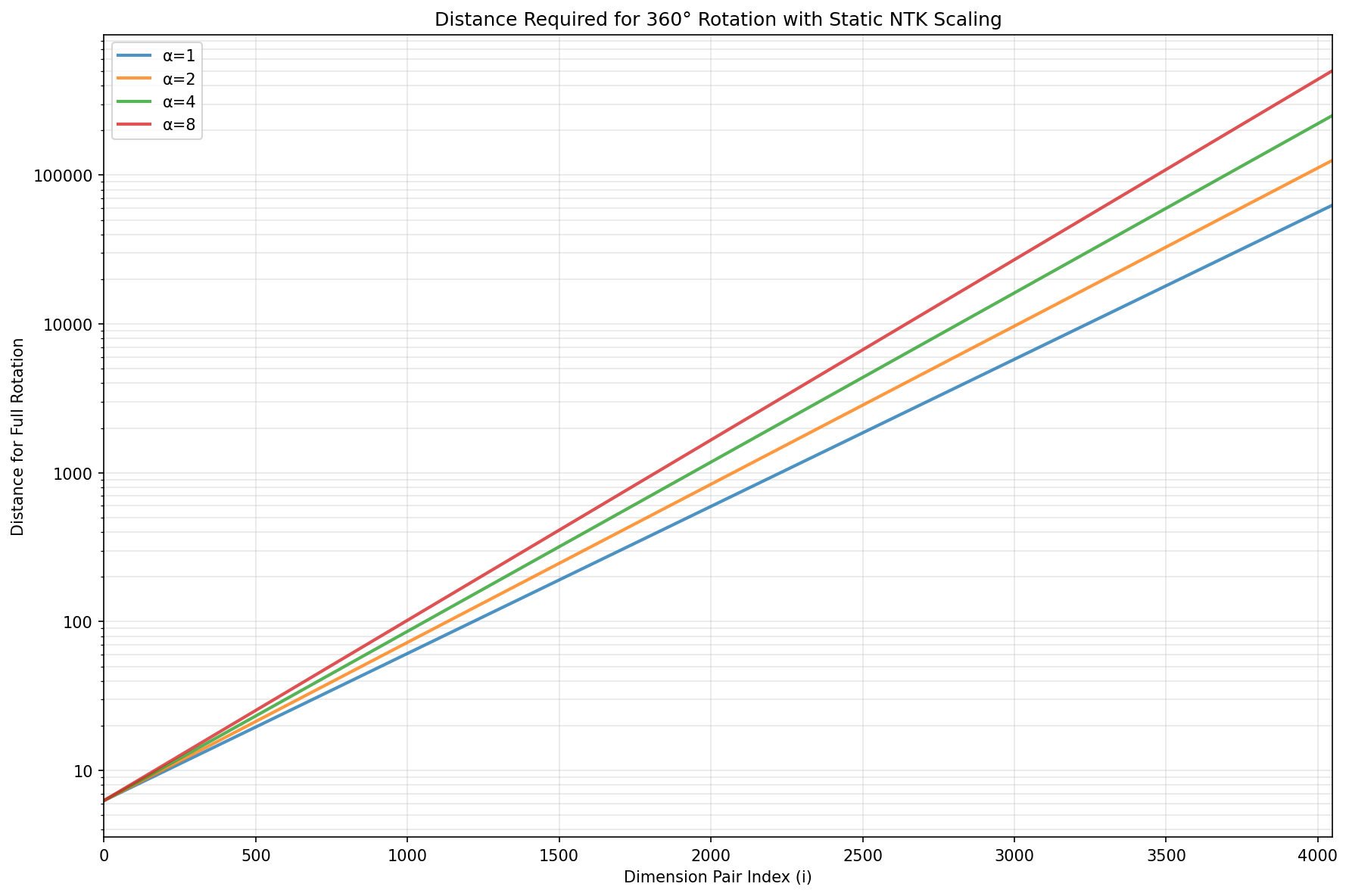
Here is another variation of the same graph. This time let’s take a look at the distance required to get a full rotation depending on the subdimension index $i$:

Finally, how does the rotation actually looks like? On the following graph we visualize pairs of $x_i, y_i$ as a vector. We start from a original vector $[1,1]$ and show how it changes for small distances of 0 to 7 for $i=[0, 60, 500, 2000, 3250]$:

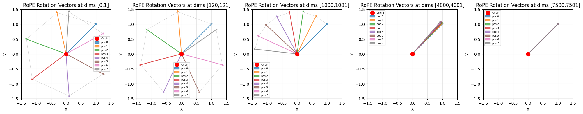
We can see that in high-i rotation is barely noticeable for small distance (p).

StaticNTK

First major known improvement (according to me) over the original RoPE was this Reddit post: NTK-Aware Scaled RoPE allows LLaMA models to have extended (8k+) context size… that people now generally refer to as $StaticNTK$. The work was inspired by NTK but knowing what NTK is redundant to understanding the proposed modified transformation:

\[\theta_i^{\mathrm{NTK}}(p) = p \cdot Q^{- \frac{2i}{d}} \cdot \boldsymbol{\alpha^{- \frac{2i}{d-2}}}\]

Static NTK introduces scaling parameter $\alpha$ with suggested values of $[2, 4, 8]$ (these are about as good). $\alpha$ has little affect on small i-indexes but high $i$-indexes would have angle $\theta$ reduced by $\alpha$.

$\alpha=1$ is equivalent to the old rope. Unfortunately, I had to abandon bar charts in favor of lines that may give a false sense of continuity of the function.

Interestingly enough, standard RoPE can be replaced with StaticNTK in inference. When given a few-shot finetuning performance degradation is negligible.

Another interesting fact is that StaticNTK is better than simply increasing Q by the same factor. To spell it out: changing $Q:10000->80000$ would yield the same smallest rotation $\theta_{4095}$ as StaticNTK with $\alpha=8$ but the curve would be different and this difference is important.

Dynamic Scaling

Dynamic NTK defines a rescaled position $\tilde{p}$:

\[\tilde{p} = \begin{cases} p, & p \le L_{\mathrm{train}} \\ p \cdot \dfrac{L_{\mathrm{train}}}{L_{\mathrm{target}}}, & p > L_{\mathrm{train}} \end{cases}\]

Then applies standard RoPE using the rescaled position:

\[\theta_i^{\mathrm{dyn}}(p) = \tilde{p} \cdot Q^{- \frac{2i}{d}}\]

Interpretation: the graphs for $\theta$ would look the same as stock RoPE, but we rescale portion of distances. Example: if we trained on sequences of maximum size 4000 and we throw a sequence of size 12000 during inference we would scale the distances greater than 4000 by $0.33=4000/12000$. To me it appears that transformations-wise words in positions $4000….12000$ would be mapped to the $1333…4000$ range.

YaRN (Yet another RoPE extensioN)

YaRN (arxiv.org/2309) heuristicizes RoPE even further. It updates attention softmax formula and applies scaling (if you squint, in may look a lot like DynamicNTK) but only to higher dimensions of embedding space (higher $i$). The paper is very information dense and we would unpack new projection in two steps not without some criminal oversimplifications.

First, attention formula update. Authors suggest replacing

\[\text{softmax}\left(\frac{q^T_m k_n}{\sqrt{|D|}}\right) \to \text{softmax}_{\text{yarn}}\left(\frac{q^T_m k_n}{t \sqrt{|D|}}\right)\]

Where the formula for temperature $t$ is a) defined as function per model and b) value $t$ is calculated per-target. For LLAMA/LLAMA2 it is said to be best selected depending on the new context length $L’$ as below. Quick synthetic experiment (not shown) suggests that as the sequence length growth this choice of curve $t$ tends to reduce the maximum attention score more aggressively.

\[t = (0.1 \ln(\frac{L_{\text{target}}}{L_{\text{train}}}) + 1)^2\]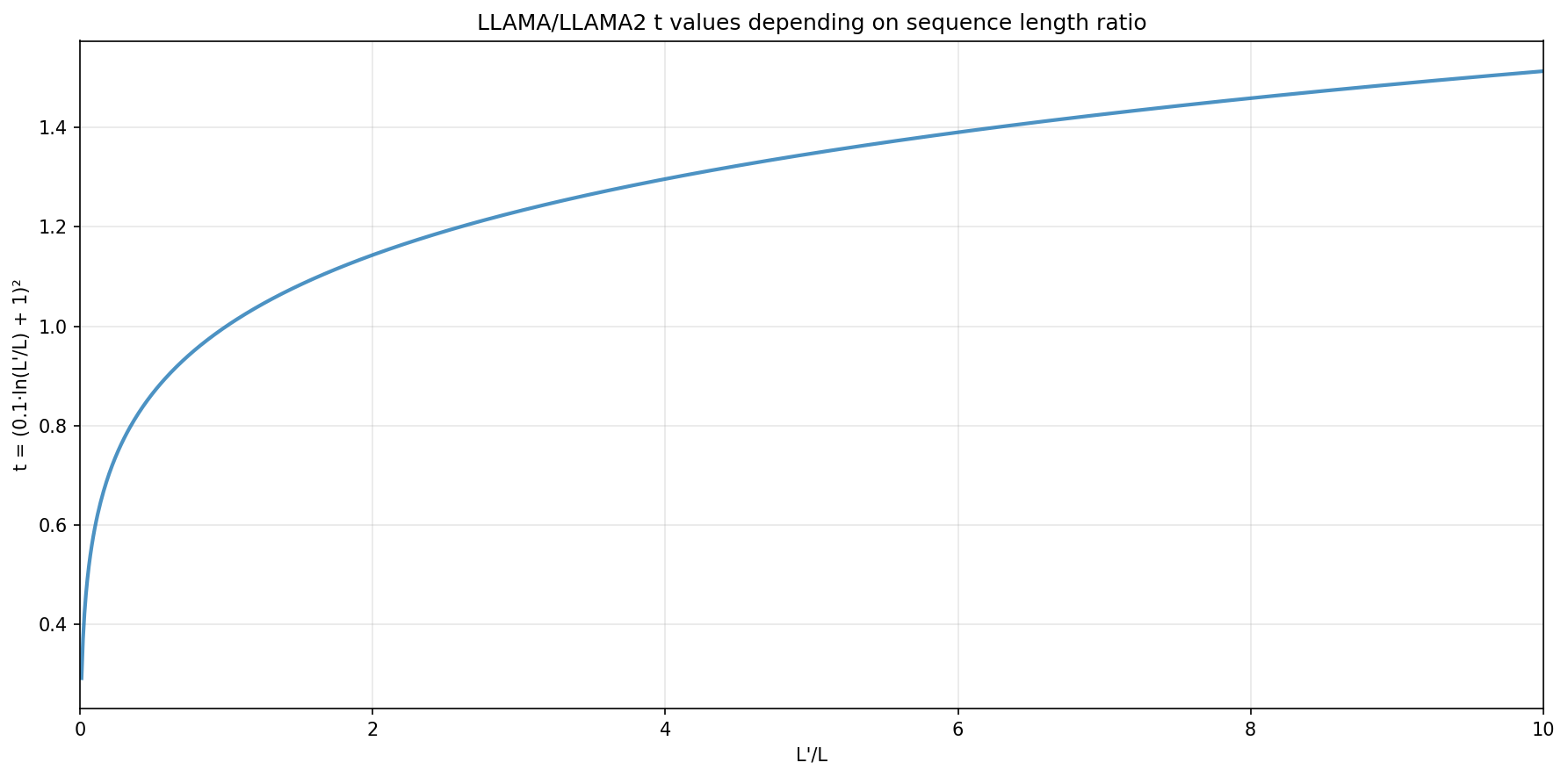

Now, to the angle rotation formula. YaRN takes indexes $i$ of the embedding dimensions (again $i\in [0, 4095]$ for embeddings size 8192) and splits them into 3 blocks: the low-$i$ (high frequency) ones are not scaled at all, middle portion is a linear transition from 100% non-scaled to 100% scaled, and the 100% scaled portion comes at the end.

The formula goes as following:

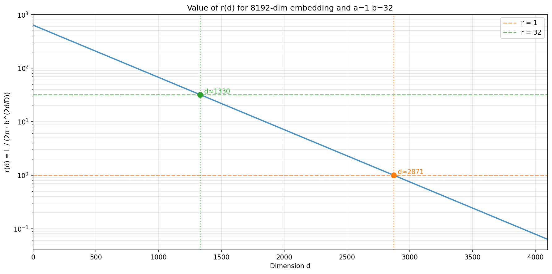
\[\gamma_i^* = \begin{cases} 0, & \text{if } i/D < d_\alpha \\[1mm] \dfrac{i/D - d_\alpha}{d_\beta - d_\alpha}, & \text{if } d_\alpha < i/D < d_\beta\\[1mm] 1, & \text{if } i/D > d_\beta \end{cases}\] \[\theta_i^{YaRN} = (1 - \gamma_i^*) \theta_i + \gamma_i^* \theta_i \frac{L_{\text{train}}}{L_{\text{target}}}\]

$d_\alpha$ and $d_\beta \in [0, 1]$ ($d_\alpha < d_\beta$) are 2 more hyperparameters for one to select. In the original paper authors actually pick parameters $\alpha$ and $\beta$ in a different subspace based on an exponential transformation $r(i)=\frac{L}{2 \pi Q^{2i/D}}$ but this makes no difference since they map bijectively to specific values of $d_\alpha$ $d_\beta$ where $0 \leq \alpha,\beta \leq D/2$. For LLAMA/LLAMA2 best suggested values happened to divide the space into 3 almost equal parts:

Some additional lingo

It maybe useful to be aware of terms such as wavelength $\lambda_i=\frac{2\pi}{\theta_i}$. And frequency $ω_i​=\frac{1}{\theta_i}$. We saw on the illustration above of $\theta$ that as index $i$ increases rotation speed decreases. One may think of $\theta_{4095}$ as the longest sinusoid: it takes the longest distance to complete one full circle i.e. this is the longest wavelength and the lowest frequency component. high i -> low rotation angle -> long wavelength -> low frequency.

LLaMA3 RoPE

LLaMA3 uses plain RoPE with a much larger base chosen at training time.
There is no NTK scaling and no position-dependent remapping. LLAMA3 trained on context length 8k.

\[\theta_i^{\mathrm{LLaMA3}}(p) = p \cdot Q_{\mathrm{L3}}^{- \frac{2i}{d}}\]

with

\[Q_{\mathrm{L3}} = 500000\]

LLAMA3.1 was trained with extended context of length 128k and does not require any handholding below this context length.